# load packages ####
library(rStrava) # devtools::install_github('fawda123/rStrava')
library(gganimate)
library(tidyverse)
library(sp)
library(ggmap)
library(raster)

# initial setup ####
# Strava key
app_name <- 'xxxx'
app_client_id <- 'xxxxx'
app_secret <- '"xxxxxxxxxxxxxxxxxxxxxxxxxxxxxxxxxxxxxxxx"'

# create strava token
my_token <- httr::config(token = strava_oauth(app_name, app_client_id, app_secret, app_scope = 'read_all,activity:read_all'))

# Google elevation API key
GoogleAPI <- 'xxxxxxxxxxxxxxxxxxxxxxxxxxxxxxxxxxxxxxx'Getting started with rStrava
rStrava is an R package that allows you to access data from Strava using the Strava API. Some of the functions of rStrava scrape data from the public Strava website but to access your own data you will need a Strava profile and an authentication token. Details on obtaining your unique token can be found on the rStrava GitHub In addition to this key, we use rgbif::elevation() to calculate the elevation of each route. This requires a Google API key which can be created here.
Got a Strava authentication token? Got a Google API key? We are ready to create some animations! To create our animations, we use gganimate that requires ImageMagick to be installed.
Loading packages and defining tokens
First load the packages that are used in the script and our Strava and Google authentication tokens. The app_scope argument in strava_oauth() has to be one of “read” , “read_all”, “profile:read_all”, “profile:write”, “activity:read”, “activity:read_all” or “activity:write”. To access your activities, activity:read_all has to be included.
A browser window should open at this point saying Authentication complete. Please close this page and return to R. This means everything is going well!
Download your data
We can then download our personal activity data using the rStrava::get_activity_list(). This function needs your strava token and your strava athlete id. For example, my strava id is 2140248.
# download strava data
my_acts <- get_activity_list(my_token)

length(my_acts)
[1] 1669This returns a large list of all your previous activities. Mine has 1028 previous entries. If you want to explore your list, you can use View(my_acts) in RStudio which opens the Data Viewer window.
Compile your data into “tidy” dataframe
rStrava has a function that compiles the information stored in the output of get_activity_list() to a “tidy” dataframe, with one row for each activity. compile_activities() finds all the columns across all activities and returns NA when a column is not present in a given activity. This means that if HR was not measured across all your strava activities, the function will still work!
# compile activities into a tidy dataframe
my_acts <- compile_activities(my_acts)

# have a look at the dataframe
dplyr::glimpse(my_acts)
Rows: 1,669
Columns: 60
$ achievement_count <dbl> 5, 9, 12, 0, 0, 1, 11, 1, 23, 3, 2, 0, 0…
$ athlete_count <dbl> 1, 1, 2, 1, 1, 1, 1, 1, 51, 1, 1, 1, 1, …
$ athlete.id <chr> "2140248", "2140248", "2140248", "214024…
$ athlete.resource_state <dbl> 1, 1, 1, 1, 1, 1, 1, 1, 1, 1, 1, 1, 1, 1…
$ average_heartrate <chr> "127.8", "127.6", "123.8", NA, "127.4", …
$ average_speed <dbl> 21.9168, 26.2476, 24.0264, 27.1476, 17.5…
$ average_temp <chr> "10", "9", "9", "7", "3", NA, NA, NA, NA…
$ average_watts <dbl> 134.7, 156.7, 148.8, 101.1, 138.1, NA, N…
$ comment_count <dbl> 1, 14, 0, 0, 0, 3, 0, 0, 3, 0, 0, 0, 2, …
$ commute <chr> "FALSE", "FALSE", "FALSE", "FALSE", "FAL…
$ device_watts <chr> "FALSE", "FALSE", "FALSE", "FALSE", "FAL…
$ display_hide_heartrate_option <chr> "TRUE", "TRUE", "TRUE", "FALSE", "TRUE",…
$ distance <dbl> 22.3615, 27.7074, 42.3477, 5.7089, 5.639…
$ elapsed_time <dbl> 3822, 3884, 6656, 757, 1158, 1923, 4469,…
$ elev_high <dbl> 73.2, 146.2, 238.6, 118.2, 126.8, 75.9, …
$ elev_low <dbl> -0.4, 2.4, 4.6, 12.8, 20.0, 68.3, 45.1, …
$ end_latlng1 <dbl> 50.15009, 50.00123, 50.15008, 50.15007, …
$ end_latlng2 <dbl> -5.084491, -5.181100, -5.084519, -5.0845…
$ external_id <chr> "garmin_ping_260217768521", "garmin_ping…
$ flagged <chr> "FALSE", "FALSE", "FALSE", "FALSE", "FAL…
$ from_accepted_tag <chr> "FALSE", "FALSE", "FALSE", "FALSE", "FAL…
$ gear_id <chr> "b11291030", "b11291030", "b11291030", "…
$ has_heartrate <chr> "TRUE", "TRUE", "TRUE", "FALSE", "TRUE",…
$ has_kudoed <chr> "FALSE", "FALSE", "FALSE", "FALSE", "FAL…
$ heartrate_opt_out <chr> "FALSE", "FALSE", "FALSE", "FALSE", "FAL…
$ id <dbl> 8566326572, 8541744691, 8531882051, 8527…
$ kilojoules <dbl> 494.9, 595.4, 944.1, 76.5, 159.9, NA, NA…
$ kudos_count <dbl> 17, 23, 14, 5, 2, 8, 27, 5, 26, 4, 11, 1…
$ location_country <chr> "United Kingdom", "United Kingdom", "Uni…
$ manual <chr> "FALSE", "FALSE", "FALSE", "FALSE", "FAL…
$ map.id <chr> "a8566326572", "a8541744691", "a85318820…
$ map.resource_state <dbl> 2, 2, 2, 2, 2, 2, 2, 2, 2, 2, 2, 2, 2, 2…
$ map.summary_polyline <chr> "a|aqHhu_^Uo@KmCOcAWo@kCwDYb@oBlEcDlC}D|…
$ max_heartrate <chr> "157", "150", "157", NA, "149", "166", "…
$ max_speed <dbl> 57.0096, 58.2696, 66.5136, 58.8420, 41.0…
$ moving_time <dbl> 3673, 3800, 6345, 757, 1158, 1878, 4314,…
$ name <chr> "Afternoon Ride", "Morning Ride. Fun unt…
$ photo_count <dbl> 0, 0, 0, 0, 0, 0, 0, 0, 0, 0, 0, 0, 0, 0…
$ pr_count <chr> "0", "1", "8", "0", "0", "0", "7", "0", …
$ private <chr> "FALSE", "FALSE", "FALSE", "FALSE", "FAL…
$ resource_state <dbl> 2, 2, 2, 2, 2, 2, 2, 2, 2, 2, 2, 2, 2, 2…
$ sport_type <chr> "Ride", "Ride", "Ride", "Ride", "Ride", …
$ start_date <chr> "2023-02-15T16:04:05Z", "2023-02-11T10:0…
$ start_date_local <chr> "2023-02-15T16:04:05Z", "2023-02-11T10:0…
$ start_latlng1 <dbl> 50.15005, 50.15006, 50.14998, 50.17089, …
$ start_latlng2 <dbl> -5.084534, -5.084494, -5.084516, -5.1274…
$ suffer_score <chr> "29", "30", "40", NA, "9", "33", "86", "…
$ timezone <chr> "(GMT+00:00) Europe/London", "(GMT+00:00…
$ total_elevation_gain <dbl> 376.0, 372.0, 601.0, 38.0, 147.0, 15.0, …
$ total_photo_count <dbl> 2, 3, 0, 0, 0, 0, 3, 0, 3, 0, 3, 0, 5, 3…
$ trainer <chr> "FALSE", "FALSE", "FALSE", "FALSE", "FAL…
$ type <chr> "Ride", "Ride", "Ride", "Ride", "Ride", …
$ upload_id <chr> "9196267205", "9168807862", "9157876592"…
$ upload_id_str <chr> "9196267205", "9168807862", "9157876592"…
$ utc_offset <chr> "0", "0", "0", "0", "0", "0", "0", "0", …
$ visibility <chr> "everyone", "everyone", "everyone", "eve…
$ workout_type <chr> "10", "10", NA, NA, NA, NA, "0", NA, "0"…
$ average_cadence <chr> NA, NA, NA, NA, NA, "79.5", "81.3", "80.…
$ location_city <chr> NA, NA, NA, NA, NA, NA, NA, NA, NA, NA, …
$ location_state <chr> NA, NA, NA, NA, NA, NA, NA, NA, NA, NA, …There are so many columns here, so I remove some columns I am not interested in for this post and do some data transformations to get the date in a correct format. I also do not want to run the example on all my rides, instead I filter them for just 2020.
# columns to keep
desired_columns <- c('distance', 'elapsed_time', 'moving_time', 'start_date', 'start_date_local', 'type', 'map.summary_polyline', 'location_city', 'upload_id')

# keep only desired columns
my_acts2 <- dplyr::select(my_acts, any_of(desired_columns))

# transformations ####
my_acts <- mutate(my_acts,
                  activity_no = seq(1,n(), 1),
                  elapsed_time = elapsed_time/60/60,
                  moving_time = moving_time/60/60,
                  date = gsub("T.*$", '', start_date) %>%
                    as.POSIXct(., format = '%Y-%m-%d'),
                  EUdate = format(date, '%d/%m/%Y'),
                  month = format(date, "%m"),
                  day = format(date, "%d"),
                  year = format(date, "%Y")) %>%
  mutate(., across(c(month, day), as.numeric)) %>%
  filter(.,year == '2020')
Get latitude and longitude for each activity
Each activity has a bunch of data associated with it. For mapping, I am interested in the map.summary_polyline, which is a Google polyline which allows the encoding of multiple latitude and longitude points as a single string. We can get the latitude and longitude for each of the activities by using get_latlon() which decodes the polylines and using dplyr and purrr to iterate over every activity in the dataframe. I add my Google API key as a column so that map() can easily find it.
# get lat lon and distance of every ride ####
lat_lon <- my_acts %>%
  filter(!is.na(map.summary_polyline)) %>%
  filter(type == 'Ride') %>%
  mutate(key = GoogleAPI) %>%
  group_by(activity_no) %>%
  nest() %>%
  mutate(coords = map(data, ~get_latlon(.$map.summary_polyline, key = .$key)),
         dist = map(coords, ~get_dists(.x$lon, .x$lat))) %>%
  unnest(., data) %>%
  unnest(., c(coords, dist))
Having got the latitude and longitude for every ride, we can now get the elevation of each point and then calculate the gradient between points. To do this I use elevation() in the R package rgbif. To use this, you need to get a GeoNames username by registering for an account at http://www.geonames.org/login.
# get elevation and calculate gradient between points
lat_lon <- ungroup(lat_lon) %>%
  mutate(., ele = rgbif::elevation(latitude = .$lat, longitude = .$lon, user = 'YOUR USERNAME HERE', model = 'srtm1')$elevation_geonames)

lat_lon <- group_by(lat_lon, activity_no) %>%
  mutate(., ele_diff = c(0, diff(ele)),
         dist_diff = c(0, diff(dist)),
         grad = c(0, (ele_diff[2:n()]/10)/dist_diff[2:n()])) %>%
  ungroup() %>%
  dplyr::select(., -c(ele_diff, dist_diff))
This now gives us a data frame of all my rides from 2020 with the latitude, longitude, cumulative distance, elevation and gradient. It would now be super easy to create elevation profiles, but I will save that for another post.
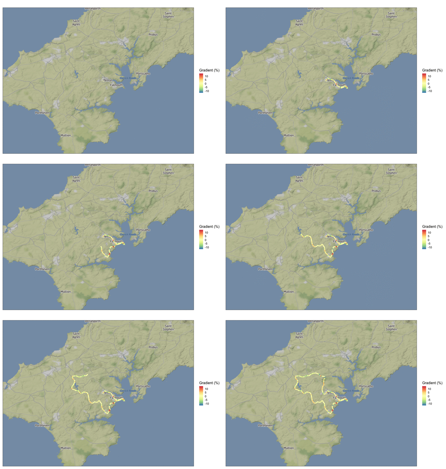
Create a gif of a single ride
We now have almost all the components to create a gif of a single ride.
lat_lon_single <- filter(lat_lon, activity_no == min(activity_no))
nrow(lat_lon_single)
[1] 343However, Google polylines do not give a consistent number of latitude and longitude points. This means it might be hard to get a smooth elevation profile for the ride and also for smooth transitions in a gif. To create a set number of points from the current polyline, we can use geospatial packages such as sp and raster to interpolate a desired number of points from the current ones. Here I create 250 points.
# reorder columns so lat lon are first
lat_lon_single <- dplyr::select(lat_lon_single, lat, lon, everything())

# make new data with by interpolation
interp <- raster::spLines(as.matrix(lat_lon_single[,1:2])) %>%
  sp::spsample(., n = 250, type = 'regular') %>%
  data.frame() %>%
  mutate(., dist = get_dists(lon, lat),
         ele = rgbif::elevation(latitude = .$lat, longitude = .$lon, user = 'padpadpadpad', model = 'srtm1')$elevation_geoname,
         ele_diff = c(0, diff(ele)),
         dist_diff = c(0, diff(dist)),
         grad = c(0, (ele_diff[2:n()]/10)/dist_diff[2:n()]),
         n = row_number())
We can now put the gif together, using ggmap and ggplot2. We use gganimate to make the plot animated.
# make bbox
bbox <- ggmap::make_bbox(lon, lat, data = lat_lon_single, f = 1.3)

# download map
map <- get_map(location = bbox, source = 'google', maptype = 'terrain')

single_ride <- ggmap(map, darken = 0.15) +
  geom_path(aes(x = lon, y = lat,  col = grad, group = 1), data = interp, size = 2, alpha = 1) +
  scale_color_distiller('Gradient (%)', palette = 'Spectral') +
  labs(title = '') +
  coord_cartesian() +
  ggforce::theme_no_axes(theme_bw(base_size = 16)) +
  transition_reveal(dist)

# animate plot
gganimate::anim_save('where_to_save.gif', single_ride, width = 1000, height = 700)
The output of this code can be seen below.

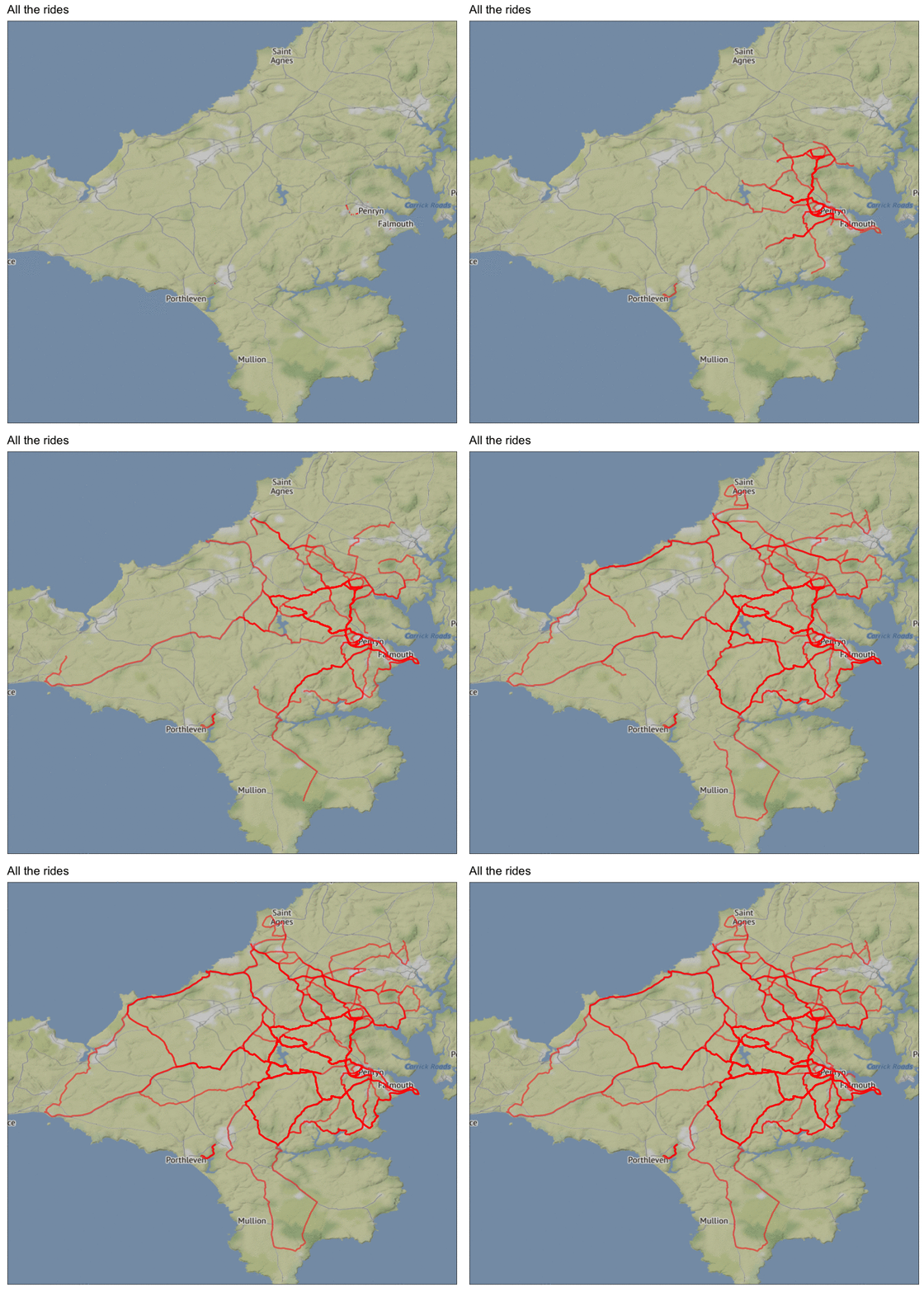
Create a gif of ALL the rides
We can also make a gif of multiple activities. I will filter my activities to only be bike rides over 15km.
# get a bbox for Cornwall
bbox <- ggmap::make_bbox(lat_lon_single$lon, lat_lon_single$lat, f = 1.2)

# add column for frame and total distance per ride
lat_lon <- group_by(lat_lon, activity_no) %>%
  mutate(n = 1:n(),
         tot_dist = max(distance)) %>%
  ungroup()

# filter lat_lon for when points are within this
lat_lon <- filter(lat_lon, between(start_longitude, bbox[1], bbox[3]) & between(start_latitude, bbox[2], bbox[4]) & type == 'Ride' & tot_dist > 15)

# add column for frame
lat_lon <- group_by(lat_lon, activity_no) %>%
  mutate(n = 1:n()) %>%
  ungroup()

# make bbox again
bbox <- ggmap::make_bbox(lon, lat, data = lat_lon, f = 0.1)

# download map
map <- get_map(location = bbox, source = 'google', maptype = 'terrain')

all_the_rides <- ggmap(map, darken = 0.15) +
  geom_path(aes(x = lon, y = lat, group = activity_no), col = 'red', data = lat_lon, size = 1.25, alpha = 0.5) +
  labs(title = 'All the rides') +
  coord_cartesian() +
  ggforce::theme_no_axes(theme_bw(base_size = 16)) +
  theme(legend.position = 'none') +
  transition_reveal(n)

# animate plot
gganimate::anim_save('where_to_save.gif', all_the_rides, width = 750, height = 700)
And there we have it. A relatively simple way to animate your strava activities in R. I personally find that saving the output as .mp4 rather than .gif gives smaller and higher quality files when uploading them to Instagram, but these options are easy to change. Take back your own data and get plotting!
There are loads of other functions and uses for the rStrava package. I hope to blog more about them soon.